Comparing Multiple Forecasters with SMCS • seqcomp

library(seqcomp)

Overview

While compare_forecasts() evaluates exactly two models, real-world applications often require comparing an arbitrary number of candidate models ( $m \ge 2$ ) simultaneously.

Evaluating multiple models sequentially introduces a multiple-testing problem: if you run enough pairwise comparisons over enough time steps, you will eventually find false “statistically significant” differences by pure chance.

To solve this, seqcomp implements Sequential Model Confidence Sets (SMCS) (Arnold et al., 2026). The SMCS is the set of models that have not yet been confidently beaten by any other model in the candidate pool. The package guarantees that the true best model(s) will remain in the SMCS with probability at least $1 - \alpha$ over the entire evaluation period. (If you are only comparing two forecasters, we recommend starting with the introductory vignette.)

Two Notions of Superiority

When comparing multiple models, seqcomp tracks two different definitions of what makes a model “superior”:

The Strong Null (smcs_strong): A model is strongly superior if it performs at least as well as every other model at every single time step. If a model is consistently good but has occasional severe failures, it will be eliminated from this set.
The Weak Null (smcs_weak): A model is weakly superior if it performs at least as well as every other model on average over time. This allows models to remain in the set even if they occasionally issue bad forecasts, provided their long-term average remains dominant.

A simple multi-model example

Let’s generate a sequence of binary outcomes and three candidate forecasters:

M1: A highly accurate forecaster.
M2: A mediocre forecaster that guesses randomly.
M3: A terrible forecaster that is consistently wrong.

set.seed(2026)
T_sim <- 300
y <- rbinom(T_sim, size = 1, prob = 0.7)

# Create 3 forecasters
forecasts <- matrix(0, nrow = T_sim, ncol = 3)
colnames(forecasts) <- c("M1", "M2", "M3")

forecasts[, "M1"] <- ifelse(y == 1, 0.8, 0.2)   # Highly accurate
forecasts[, "M2"] <- runif(T_sim, 0.4, 0.6)     # Mediocre/random
forecasts[, "M3"] <- ifelse(y == 1, 0.2, 0.8)   # Consistently wrong

head(forecasts)
#>       M1        M2  M3
#> [1,] 0.8 0.5019408 0.2
#> [2,] 0.8 0.5009826 0.2
#> [3,] 0.8 0.5262100 0.2
#> [4,] 0.8 0.4685904 0.2
#> [5,] 0.8 0.5677538 0.2
#> [6,] 0.8 0.4215049 0.2

Compare the forecasts

The easiest workflow for evaluating three or more models is to use compare_multiple_forecasts().

multi_cmp <- compare_multiple_forecasts(
  forecasts = forecasts,
  outcomes = y,
  scoring_rule = "brier",
  alpha = 0.05
)

# Printing the object provides a clean summary of which models 
# were excluded and when they first dropped out of the set.
multi_cmp
#> <seqcomp multi-model comparison>
#>   3 models, 300 time steps, alpha = 0.05, scoring rule = 'brier'
#> 
#> -- Strong-null SMCS (Permanent Exclusion) --
#>  model status_at_T first_dropped
#>     M1    included             -
#>     M2    excluded            87
#>     M3    excluded            33
#>    final set size: 3 -> 1
#> 
#> -- Weak-null SMCS (Dynamic Re-entry) --
#>  model status_at_T first_dropped
#>     M1    included             -
#>     M2    excluded            61
#>     M3    excluded            22
#>    final set size: 3 -> 1
#> 
#> Use `x$smcs_strong` / `x$smcs_weak` for full inclusion matrices, or `x$scores` for pointwise scores.

While the printed summary gives a quick overview, the underlying object is a list containing the full time-indexed matrices for further analysis(alongside metadata such as alpha and scoring_rule):

multi_cmp$scores: The evaluated pointwise scores for each model.
multi_cmp$smcs_strong: A logical matrix tracking whether each model belongs to the strong-null SMCS at time $t$ .
multi_cmp$smcs_weak: A logical matrix tracking whether each model belongs to the weak-null SMCS at time $t$ .

Interpreting the SMCS output

smcs_strong() maintains a running intersection over time: once a model is shown to violate the null against some competitor, it is excluded permanently. This matches the strong/uniformly-weak SMCS construction of Arnold, Gavrilopoulos, Schulz and Ziegel (2026, Section 3.2).

The underlying hypothesis of smcs_weak() (the time-varying weak null, Section 3.3) is defined at each time $t$ , not cumulatively, so a model’s average performance can legitimately recover after a bad stretch. smcs_weak() therefore returns smcs, which can re-admit models that were previously excluded.

Let’s look at the strong SMCS at the end of the evaluation:

tail(multi_cmp$smcs_strong)
#>          M1    M2    M3
#> [295,] TRUE FALSE FALSE
#> [296,] TRUE FALSE FALSE
#> [297,] TRUE FALSE FALSE
#> [298,] TRUE FALSE FALSE
#> [299,] TRUE FALSE FALSE
#> [300,] TRUE FALSE FALSE

We can visualize how the confidence set shrinks over time by plotting whether a model is TRUE (Included) or FALSE (Excluded):

par(mfrow = c(3, 1), mar = c(2, 4, 2, 1))
colors <- c("blue", "gray", "red")

for (i in 1:3) {
  plot(
    1:T_sim, multi_cmp$smcs_strong[, i], 
    type = "s", col = colors[i], lwd = 2,
    ylim = c(-0.1, 1.1), yaxt = "n", ylab = "In SMCS?",
    main = paste("Model:", colnames(forecasts)[i])
  )
  axis(2, at = c(0, 1), labels = c("Excluded", "Included"), las = 2)
}

par(mfrow = c(1, 1))

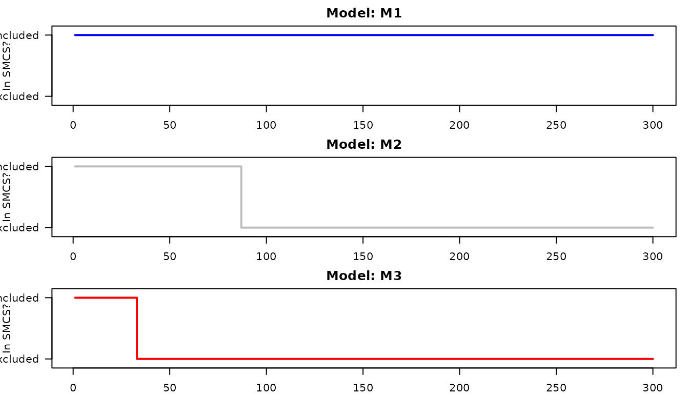
Notice how quickly the set shrinks:

M3 (the terrible model) is confidently beaten by M1 almost immediately and drops out of the set.
M2 (the mediocre model) survives a bit longer, but as evidence accumulates, it too is permanently excluded.
M1 (the true best model) remains in the SMCS for the entire duration.

Using lower-level functions directly

Just like the two-model case, seqcomp exposes the underlying multi-model primitives if you need custom bounds, different scoring rules, or adaptive betting fractions.

You can compute your own score matrices and pass them directly to smcs_strong() or smcs_weak().

# Manually compute Brier scores
scores_mat <- matrix(0, nrow = T_sim, ncol = 3)
for(i in 1:3) scores_mat[, i] <- brier_score(forecasts[, i], y)

# Construct the Weak SMCS directly
# Brier score differences are bounded in [-1, 1], so we use c_param = 2
res_weak <- smcs_weak(
  scores = scores_mat,
  alpha = 0.05,
  cs_method = "bernstein",
  c_param = 2
)

tail(res_weak$smcs)
#>        [,1]  [,2]  [,3]
#> [295,] TRUE FALSE FALSE
#> [296,] TRUE FALSE FALSE
#> [297,] TRUE FALSE FALSE
#> [298,] TRUE FALSE FALSE
#> [299,] TRUE FALSE FALSE
#> [300,] TRUE FALSE FALSE

Conditionally bounded scores (Tick loss)

Some scoring rules, like tick loss for quantile forecasting, are unbounded globally but bounded conditionally based on the distance between the forecasts.

For these rules, the strong SMCS requires a dynamically updating 3D array of bounds and betting fractions. The wrapper compare_multiple_forecasts() handles this automatically when scoring_rule = "tick", or you can construct the arrays manually using build_quantile_betting_arrays().

set.seed(7)
tau <- 0.5

truth <- rnorm(T_sim)
q_forecasts <- cbind(
  M1 = truth + rnorm(T_sim, sd = 0.1),    # accurate
  M2 = rep(0, T_sim),                     # uninformative
  M3 = truth + rnorm(T_sim, sd = 0.1) + 1 # biased
)

tick_cmp <- compare_multiple_forecasts(
  forecasts    = q_forecasts,
  outcomes     = truth,
  scoring_rule = "tick",
  tau          = tau,
  alpha        = 0.05
)
#> Warning in compare_multiple_forecasts(forecasts = q_forecasts, outcomes =
#> truth, : smcs_weak is currently omitted for unbounded tick loss in this wrapper
#> (requires transformation).

tail(tick_cmp$smcs_strong)
#>          M1    M2    M3
#> [295,] TRUE FALSE FALSE
#> [296,] TRUE FALSE FALSE
#> [297,] TRUE FALSE FALSE
#> [298,] TRUE FALSE FALSE
#> [299,] TRUE FALSE FALSE
#> [300,] TRUE FALSE FALSE

smcs_weak is NULL here, since tick-loss score differences are only conditionally bounded, not uniformly bounded, and smcs_weak() currently requires a fixed uniform bound.