Choosing an Adaptive Betting Strategy: Temporal Dependence and Pathologies • seqcomp

library(seqcomp)

Introduction

smcs_strong(method = "betting") tests the strong null through a product-form martingale, $E_t = \prod_{r \le t} (1 + \lambda_r d_r)$ , where $d_r$ is a score difference and $c_r$ is a predictable bound with $|d_r| \le c_r/2$ . Validity only requires that $\lambda_r$ be predictable and lie in $[0, 1/c_r]$ at every round (see the SMCS vignette for the underlying construction). Everything else, how large $\lambda_r$ actually is on a given round, is a design choice, and that choice determines how fast the test can reject a genuinely worse model.

seqcomp ships four ways to make that choice:

the conservative fixed fraction $\lambda_t = 1/(2c_t)$ , the package default,
lambda_betting_agrapa(), an adaptation of Waudby-Smith and Ramdas (2024)’s aGRAPA plug-in,
lambda_betting_ons(), an adaptation of their ONS-m online Newton step,
lambda_betting_quantile(), Arnold et al. (2026)‘s own arctangent heuristic for quantile forecasts (referred to here as ’Arnold’s heuristic’ for brevity, though derived jointly by Arnold, Gavrilopoulos, Schulz, and Ziegel, 2026).

Arnold et al. (2026) do not define or recommend either aGRAPA or ONS-m; both are adaptations original to this package, built for a different null than the one Waudby-Smith and Ramdas (2024) designed them for (see the roxygen documentation for lambda_betting_agrapa() and lambda_betting_ons() for the derivation). None of the four rules is a strict improvement on the others. Each one responds differently to the observed history of the score differences, and therefore performs differently under different temporal structures. This vignette walks through four scenarios where that assumption breaks down for at least one method, drawn from the package’s systematic taxonomy of betting rules (simulations/sim_06_systematic_taxonomy.R, which also carries exhaustive Type-I error checks and hyperparameter sweeps not reproduced here).

A fifth method, an oracle bet, appears in a few of the tables below purely as a ceiling. It uses the true, otherwise unobservable conditional mean and variance of the simulated data-generating process to solve directly for a highly optimized bet. It is there only to show how much room the adaptive rules leave on the table.

As these scenarios will show, there is no single ‘best’ rule because these algorithms optimize different aspects of the sequential evidence process. Some maximize terminal wealth, others minimize time-to-rejection, and others trade away power to strictly limit maximum drawdown (the largest peak-to-trough drop in the e-process from a previous high). The choice depends entirely on which of these objectives matters most for your application.

Surfing Momentum

Autocorrelated noise and a structural break are the same underlying problem at two different timescales: a running summary of the past is a poor guide to what happens next, either continuously, because rounds are correlated, or suddenly, because the mean has moved. lambda_betting_agrapa() and lambda_betting_ons() both track a running estimate, but differently, and that difference shows up clearly here.

aGRAPA is a regularized cumulative average. Its plug-in mean and variance are (prior + cumsum(...)) / (t + fake_obs), so a new observation’s weight on the estimate shrinks as $1/t$ . ONS-m instead takes a local Newton step every round, moving its bet in the direction of the current gradient and scaling the step by the accumulated curvature $A_t$ . It still pools information over the whole run through $A_t$ , but the direction of each step comes from the most recent observation, not from a long-run average.

A single path

This plot simulates one path with a mean that jumps from 0.10 to 0.40 at $t = 600$ , and traces the resulting $\lambda_t$ for both rules.

set.seed(2027)
T_sim <- 1000
c_t <- rep(2, T_sim)
mu  <- ifelse(seq_len(T_sim) <= 600, 0.10, 0.40)
d_t <- pmin(pmax(mu + rnorm(T_sim), -c_t / 2), c_t / 2)

lam_agrapa <- lambda_betting_agrapa(d_t, c = c_t)
lam_ons    <- lambda_betting_ons(d_t, c = c_t)

plot(seq_len(T_sim), lam_agrapa, type = "l", col = "red",
     xlab = "t", ylab = expression(lambda[t]),
     main = "One simulated path: betting fraction around a break at t = 600")
lines(seq_len(T_sim), lam_ons, col = "orange")
abline(v = 600, col = "blue", lty = 3)
legend("topleft", legend = c("aGRAPA", "ONS-m"), col = c("red", "orange"),
       lwd = 1, bty = "n")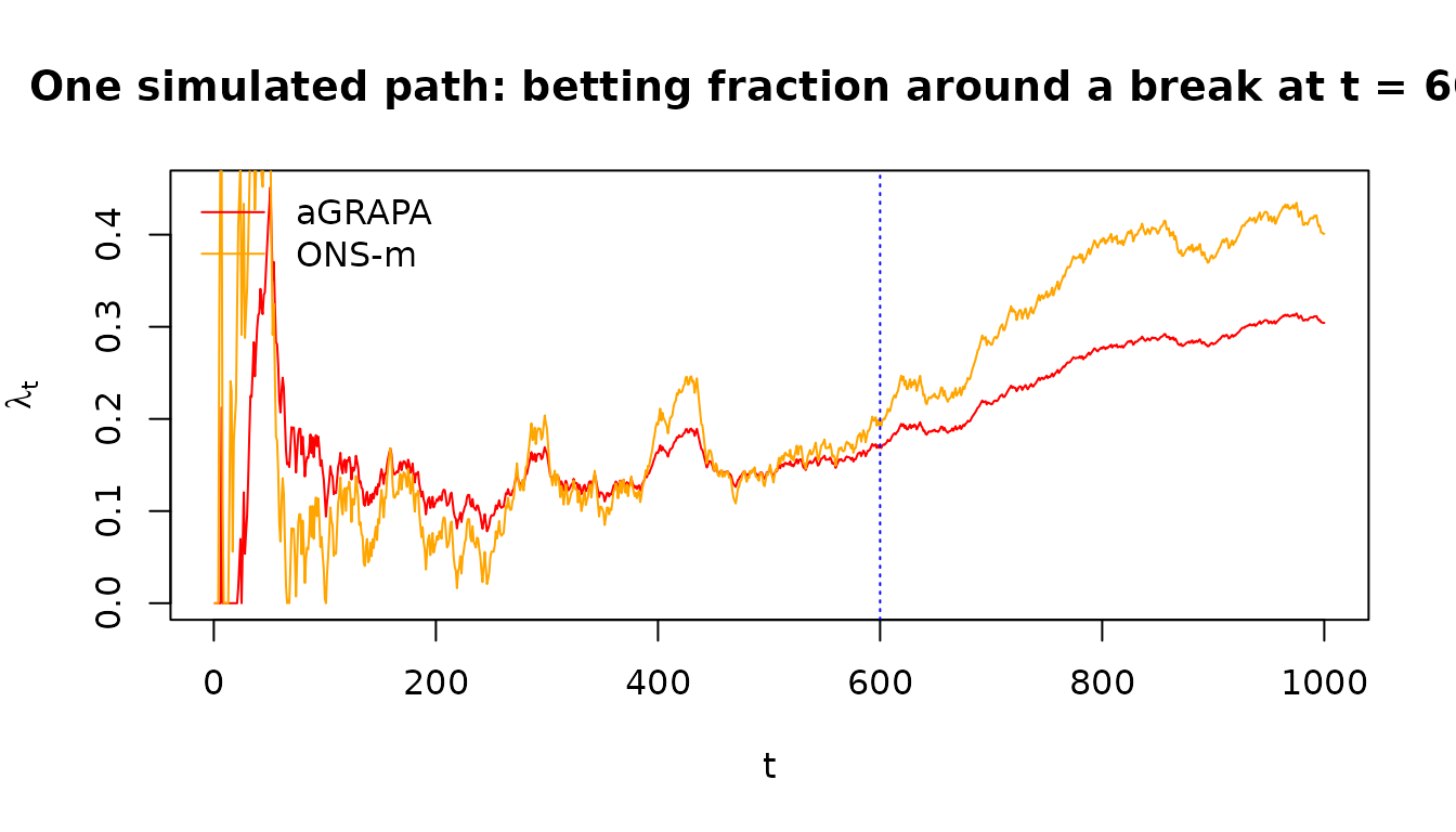

One path is not evidence. The tables below aggregate 200 runs of the same design (T = 1000, break at t = 600, c_t = 2 throughout):

simulate_dt <- function(T_, mu_fn, c_fn, rho = 0, sd_scale = 1) {
  mu  <- vapply(seq_len(T_), mu_fn, numeric(1))
  c_t <- vapply(seq_len(T_), c_fn, numeric(1))
  eps <- numeric(T_)
  eps[1] <- rnorm(1, sd = sd_scale)
  for (t in 2:T_) {
    eps[t] <- rho * eps[t - 1] + rnorm(1, sd = sd_scale * sqrt(1 - rho^2))
  }
  d_t <- pmin(pmax(mu + eps, -c_t / 2), c_t / 2)
  list(d_t = d_t, c_t = c_t)
}

mu_break   <- function(t) if (t <= 600) 0.10 else 0.40
c_const_fn <- function(t) 2.0

N_runs <- 200
T_sim  <- 1000
lam_pre  <- matrix(NA, N_runs, 2, dimnames = list(NULL, c("aGRAPA", "ONS-m")))
lam_post <- lam_pre

for (sim in seq_len(N_runs)) {
  dat   <- simulate_dt(T_sim, mu_break, c_const_fn, rho = 0, sd_scale = 1)
  lam_a <- lambda_betting_agrapa(dat$d_t, c = dat$c_t)
  lam_o <- lambda_betting_ons(dat$d_t, c = dat$c_t)
  lam_pre[sim, ]  <- c(mean(lam_a[400:600]),  mean(lam_o[400:600]))
  lam_post[sim, ] <- c(mean(lam_a[800:1000]), mean(lam_o[800:1000]))
}

colMeans(lam_pre)   # average bet just before the break
colMeans(lam_post)  # average bet well after the break

Mean betting fraction, averaged over the 200 runs, just before the break ( $t \in [400, 600]$ ) and well after it ( $t \in [800, 1000]$ ):

Method	Pre_break	Post_break
Oracle	0.132	0.494
ONS-m	0.139	0.353
aGRAPA	0.132	0.255
Naive	0.250	0.250

Naive does not move, by construction. Both adaptive rules raise their bet after the break, but ONS-m’s post-break fraction sits noticeably closer to the oracle’s than aGRAPA’s does.

One could expect the opposite result, as ONS-m’s Hessian proxy $A_t = 1 + \sum z_i^2$ never decreases, so it seems reasonable to guess that a long run of pre-break history would leave ONS-m’s effective step size too small to react quickly once the break hit, a staleness that aGRAPA’s simpler running average would not share. Post-break wealth multipliers at four different break points refute such a guess directly:

Break t*	aGRAPA post-break multiplier	ONS-m post-break multiplier
100	1.975e+37	7.295e+37
300	6.554e+24	8.168e+27
600	1.567e+11	6.591e+13
800	2.920e+04	3.626e+05

At every break point tested, ONS-m compounds more wealth after the break than aGRAPA does. The mechanical reason lies in how they update. aGRAPA’s mean and variance estimates retain the influence of the entire history, so a break at $t = 800$ still has to fight against 800 rounds of stale pre-break data. ONS-m’s step direction, by contrast, is local, as it reacts to the current gradient, even though its step size is scaled by the accumulated curvature $A_t$ . This allows it to pivot faster. The staleness hypothesis was a reasonable guess from the formula alone, but it does not survive running the two rules side by side.

On the other hand, median maximum drawdown in the same 200-run design was 13.90 for aGRAPA against 18.13 for ONS-m: aGRAPA’s slower reaction also buys a gentler ride in this particular design, and ONS-m’s willingness to move its bet further, faster, is what produces the larger post-break payoff.

Autocorrelated noise pushes in the same direction without any break at all. These runs generated an AR(1) noise process around a mean of 0.05, and then clipped the resulting score difference to the admissible $[-c_t/2, c_t/2]$ range at three levels of persistence:

rho_vals <- c(0.0, 0.5, 0.9)
N_runs <- 200
T_sim  <- 1000
get_mdd <- function(e) max(cummax(e) / e)

for (r in rho_vals) {
  final_e <- matrix(NA, N_runs, 2, dimnames = list(NULL, c("aGRAPA", "ONS-m")))
  mdd     <- final_e
  for (sim in seq_len(N_runs)) {
    dat   <- simulate_dt(T_sim, mu_fn = function(t) 0.05, c_fn = function(t) 2.0,
                         rho = r, sd_scale = 1.0)
    lam_a <- lambda_betting_agrapa(dat$d_t, c = dat$c_t)
    lam_o <- lambda_betting_ons(dat$d_t, c = dat$c_t)
    e_a   <- cumprod(1 + lam_a * dat$d_t)
    e_o   <- cumprod(1 + lam_o * dat$d_t)
    final_e[sim, ] <- c(e_a[T_sim], e_o[T_sim])
    mdd[sim, ]     <- c(get_mdd(e_a), get_mdd(e_o))
  }
  # medians reported in the table below
}

$\rho$	aGRAPA final wealth	ONS-m final wealth	aGRAPA drawdown	ONS-m drawdown
0.0	0.44	0.36	11.52	26.29
0.5	0.80	43.6	75.22	72.71
0.9	1.08	1.15852e+12	98,600.77	30,731.16

(Naive ends near zero at every $\rho$ tested under this weak, mean-0.05 signal, and the oracle’s final wealth is orders of magnitude larger still, since it knows the true mean and variance directly.)

Under i.i.d. noise ( $\rho = 0.0$ ), neither adaptive method compounds meaningfully, both end below where they started, and aGRAPA has the lower drawdown here. Once real persistence enters at $\rho = 0.5$ , ONS-m’s final wealth overtakes aGRAPA’s by roughly 54 times, and at $\rho = 0.9$ the gap is no longer a multiple, but a difference in scale. Under this specific simulation design, if the score difference stream carries strong serial correlation, ONS-m’s local gradient updating proved to be a much more powerful default than aGRAPA’s pooled estimates.

The Micro-Variance Trap

lambda_betting_quantile()’s bound $c_t = 2\max(\tau, 1-\tau)|p_t - q_t|$ scales with the distance between the two forecasts, which shifts the focus to quantile forecasts evaluated under tick loss. When two models are nearly identical, which is common once a Sequential Model Confidence Set has narrowed to its final few survivors, $c_t$ collapses toward zero, and the naive rule’s ceiling $\lambda_t = 1/(2c_t)$ explodes in the opposite direction.

Tier B, Test 4 of the taxonomy pushes this to an extreme: two median forecasters ( $\tau = 0.5$ ) that differ by only $\pm 0.001$ around the same GARCH-simulated series.

simulate_garch <- function(T_, omega = 0.05, alpha = 0.15, beta = 0.80) {
  y <- sigma2 <- numeric(T_)
  sigma2[1] <- omega / (1 - alpha - beta)
  y[1] <- rnorm(1, sd = sqrt(sigma2[1]))
  for (t in 2:T_) {
    sigma2[t] <- omega + alpha * y[t - 1]^2 + beta * sigma2[t - 1]
    y[t] <- rnorm(1, sd = sqrt(sigma2[t]))
  }
  list(y = y, sigma = sqrt(sigma2))
}

set.seed(2029)
T_sim <- 1000
dgp <- simulate_garch(T_sim)

q_oracle <- rep(0, T_sim)
q_micro  <- q_oracle + 0.001 * rep(c(1, -1), T_sim / 2)

d_t <- tick_loss(q_oracle, dgp$y, tau = 0.5) - tick_loss(q_micro, dgp$y, tau = 0.5)

delta_lag1 <- c(0, head(d_t, -1))
bnds <- lambda_betting_quantile(q_oracle, q_micro, tau = 0.5,
                                delta_hat_lag1 = delta_lag1)
c_t <- pmax(bnds$c_t, 1e-8)

lam_naive  <- 1 / (2 * c_t)
lam_arnold <- pmin(bnds$lambda_t, 1 / c_t)
lam_agrapa <- lambda_betting_agrapa(d_t, c = c_t)
lam_ons    <- lambda_betting_ons(d_t, c = c_t)

The average bound over the run was $c_t \approx 0.001$ , putting the naive ceiling at $\lambda \approx 500$ . Average betting fraction actually played, and terminal wealth at $t = 1000$ :

Method	Average $\lambda_t$ played	Terminal wealth
Naive	500.0	0.0
Arnold	333.3	0.0
aGRAPA	5.0	0.2
ONS-m	70.8	0.0

In this run, naive, Arnold’s heuristic, and ONS-m all played very large bets relative to the optimal fraction and ended with essentially zero wealth. ONS-m’s average bet (70.8) was much lower than naive’s, but still vastly more aggressive than aGRAPA’s, which was enough to trigger catastrophic volatility drag. aGRAPA is the only method that retained non-negligible wealth.

The reason traces to the fact that aGRAPA contains an explicit prior_variance regularization term that keeps its plug-in denominator away from zero even when the empirical signal is tiny. The other three betting rules do not impose this kind of variance regularization, allowing their bets to escalate dangerously in high-noise, low-signal regimes.

Riding the ceiling is fragile in a specific, checkable way. A bet at exactly $\lambda = 1/c$ multiplies wealth by $1 + (1/c)(-c/2) = 1/2$ on the single worst possible draw, confirmed directly on a deliberately constructed single-shock path elsewhere in the taxonomy script: aGRAPA and ONS-m each lost exactly 50% of their wealth on a maximal adverse observation while parked at that ceiling, while naive, betting more conservatively at $\lambda = 1/(2c)$ , lost only 25%. Algorithms that persistently play very large fractions, as naive, Arnold’s heuristic, and ONS-m all did on this path, pay that price over and over.

Volatility Clustering

Tier B, Test 3 keeps the same GARCH structure but removes the microscopic bound: one model tracks the true conditional median exactly, the other forecasts a constant 0.5 regardless of what the volatility process is doing (same harness as above, with q_static <- rep(0.5, T_sim) in place of q_micro). As volatility clusters, the score difference swings hard in both directions before eventually favoring the correct forecaster.

Terminal wealth and maximum drawdown at $t = 1000$ :

Method	Terminal wealth	Maximum drawdown
Naive	1.207e+16	19.11
Arnold	9.728e+12	5.51
aGRAPA	1.465e+15	65.23
ONS-m	9.792e+14	69.90

Arnold’s heuristic ends this run with roughly a thousand times less wealth than naive, aGRAPA, or ONS-m, and it has, by a wide margin, the smallest drawdown of the four. aGRAPA and ONS-m both compound faster and both pay for it with drawdowns an order of magnitude larger than Arnold’s. Because their bet sizes are driven by running variance estimates that lag behind sudden GARCH volatility spikes, they over-bet into the whipsaw. Arnold’s heuristic recomputes its bet directly from the current spread between the two forecasts on every round, without accumulating a running summary of the past at all, so it reacts immediately when a volatility spike passes and the spread narrows again. It behaves like a shock absorber rather than a wealth-maximizer.

This matches the broader pattern from the taxonomy: Arnold’s heuristic, purpose-built for the smooth, slowly varying, mean-reverting structure of the quantile forecasts it was designed around, is a strong choice exactly there, but it gives up compounding wealth in exchange for that stability once the process gets choppier. None of the four methods showed inflated Type-I error in the same GARCH setting under an exact null (identically noisy trackers, $\tau = 0.5$ ): naive rejected 3.6% of the time, Arnold 3.0%, aGRAPA 2.2%, and ONS-m 2.6%, all at or under the nominal 5% level, so the choice here is genuinely about power and drawdown, not validity.

The Cost of Multiplicity

Everything so far compares two models. smcs_strong() extends the same betting martingale to $m$ models via closed testing: for each model $i$ , an intersection e-process $E_{i\cdot,t}$ averages the pairwise e-processes against all $m - 1$ competitors, and a Vovk-Wang merge (vovk_wang_merge()) adjusts $E_{i\cdot,t}$ for the multiplicity of testing every model against every other model at once. The adjusted value $E^\star_{i\cdot,t}$ is a minimum over subsets of competitors, and the full set is always one candidate subset, so $E^\star_{i\cdot,t}$ can never exceed the plain average across all $m - 1$ pairwise e-processes. Adding more models whose pairwise e-processes carry little or no evidence pulls that average down and delays rejection. No choice of $\lambda_t$ changes this; it is a property of the closed-testing average itself.

A deterministic construction makes the mechanism visible without any noise: one model that fails every seventh round (a stand-in for a weekly seasonal shock) against a competitor that never fails, diluted by a growing number of models that fail every round and carry no information at all.

T_sim <- 1000
alpha <- 0.10
sundays <- seq(7, T_sim, by = 7)
m_vals <- c(2, 5, 15, 30, 49)

for (m_curr in m_vals) {
  scores_mat <- matrix(0, nrow = T_sim, ncol = m_curr)
  scores_mat[, 1] <- 1.0
  scores_mat[sundays, 1] <- 0.0   # fails every seventh round
  scores_mat[, 2] <- 1.0          # never fails
  if (m_curr > 2) scores_mat[, 3:m_curr] <- 0.0   # uninformative decoys

  C_mat <- matrix(2.0, nrow = m_curr, ncol = m_curr)
  lam_agrapa <- build_agrapa_betting_array(scores_mat, c_mat = C_mat, period = 7)
  lam_ons    <- build_ons_betting_array(scores_mat, c_mat = C_mat, period = 7)

  res_agrapa <- smcs_strong(scores_mat, alpha = alpha, method = "betting",
                            c_param = C_mat, lambda_param = lam_agrapa)
  res_ons    <- smcs_strong(scores_mat, alpha = alpha, method = "betting",
                            c_param = C_mat, lambda_param = lam_ons)
  # round of exclusion for model 1 reported below
}

period = 7 conditions each adaptive rule on its own day-of-week sub-stream instead of pooling across all seven days at once, the same construction used for the periodic seasonal example in the SMCS vignette; without it, the rules fail to react to the weekly pattern for the same pooling reason discussed above. Round at which the seasonal model is excluded, as $m$ grows:

$m$	aGRAPA (period 7)	ONS-m (period 7)	Naive
2	63	63	98
5	84	84	140
15	105	105	182
30	119	119	203
49	126	126	217

aGRAPA and ONS-m tie exactly here, since the DGP is deterministic and the periodic wrapper removes the timing advantage that separated them under noise. Naive falls behind at every value of $m$ , and the gap widens as $m$ grows: 35 rounds at $m = 2$ , 91 rounds at $m = 49$ .

A stochastic version of the same design, run 50 times per value of $m$ with an analytically derived, not data-peeked, predictable bound, gives the median rejection round:

$m$	aGRAPA (median $t$ )	ONS-m (median $t$ )	Naive (median $t$ )
2	217.0	280.0	497
10	301.0	420.0	836.5
25	346.5	439.0	868.5
49	339.5	472.5	>1,000

The overall pattern under noise is the same: increasing $m$ generally delays rejection, with the largest degradation for the naive rule. aGRAPA’s slight dip at $m=49$ should be interpreted as finite-sample noise across the 50 runs.

The dilution mechanism is exact enough to verify arithmetically. aGRAPA’s terminal wealth hits the package’s internal clip_max computational safeguard of $10^7$ per pairwise e-process. Once the closed-testing average sets in, that ceiling gets divided almost exactly by $m - 1$ :

$m$	Arnold: round of exclusion	aGRAPA: round of exclusion	aGRAPA final adjusted e-value
2	>8,000	1,786	1e+07
10	>8,000	2,516	1,111,111
25	>8,000	2,540	416,666.9
49	>8,000	2,561	208,333.6

At every $m$ tested, aGRAPA’s final adjusted e-value matches $10^7/(m-1)$ to the precision shown: the closed-testing average is literally dividing the maximum possible pairwise evidence among the competitors it is pooled against. Arnold’s heuristic never rejects within the 8000-round horizon in this setting, a separate finding from the volatility-clustering result above and consistent with it: Arnold’s heuristic does not accumulate wealth quickly against a slow-moving, well-separated competitor over a long horizon, and the dilution tax here only makes that slower accumulation worse.

Choosing a good $\lambda_t$ rule buys real power, as the sections above show, but it does not undo the cost of testing more models at once. That cost is a property of the closed-testing correction, not of the betting rule sitting underneath it, and it sets a practical limit on how large a candidate pool you should evaluate at a fixed horizon, regardless of which betting rule you pick. Exhaustive Type-I error checks and hyperparameter sensitivity sweeps for all four rules, across constant, time-varying, and periodic bound regimes, are in simulations/sim_06_systematic_taxonomy.R in the package source and are not reproduced in this vignette.

Summary

No single rule dominates across every regime tested. As a rough guide:

Situation observed in these simulations	Reasonable starting point
Autocorrelated or abrupt mean shift	ONS-m
Nearly identical models (tiny $c_t$ )	aGRAPA
Strong volatility clustering	Naive or Arnold’s heuristic (if drawdown matters)
Smooth, slowly varying, mean-reverting quantile forecasts	Arnold’s heuristic

Whatever rule you choose, expect rejection to take longer as the candidate pool $m$ grows. That cost comes from the closed-testing correction in smcs_strong(), not from the betting rule, and no choice of $\lambda_t$ removes it.